Yesterday, I attended the first day of the Astrobiology Science Conference, or AbSciCon. The day began with a great talk by Lord Martin Rees, who is the Astronomer Royal in England. He wrote a book called “Just Six Numbers” about six parameters of our solar system and Earth that have allowed for conditions conducive to the existence of life (and human beings). He was introduced by Paul Davies, who wrote “The Goldilocks Enigma”. Both books are now candidates for inclusion in my to-read list.
I next attended some talks about the galactic habitable zone. While I’ve read about the “habitable zone” inside our solar system (largely determined by the temperature range within which water exists as a liquid), this was the first time I’d encountered its galactic counterpart. In the galaxy, the constraints relevant for habitability (specifically, the creation of planets) involve the probability of a nearby, disruptive, supernova (so you don’t want to be too close to the galactic center, where stellar density is high) and the availability of metals for forming planets, which are more available where stellar density is high since they’re created by stars (so you don’t want to be too far away from the core). Our Sun is at 8.5 kiloparsecs from the galactic center, although it apparently wobbles in and out a bit, and there’s enough uncertainty in the measurement that it’s more like 7.5 to 8.8 kpc.
 The discovery of exoplanets (planets outside our solar system, orbiting other stars) is, in my opinion, one of the foremost scientific discoveries of the past decade or so. It sounds like science fiction, but it’s real (we’re up to 287 exoplanets so far!). So far we’ve predominantly found only Jupiter-sized planets that are close to their host stars (and very, very hot), but most expect that this is because those are the planets that are easiest to detect. The hunt is on for Earth-sized planets that reside in their star’s habitability zone. In particular, a five-year study is beginning to collect 100,000 observations of Alpha Centauri B in hopes of detecting terrestrial planets. No planets have yet been detected in the complex (triple star!) Alpha Centauri system. However, in planet formation simulations, 42% of the Earth-sized planets that formed fell into the habitable zone around Alpha Centauri B. Therefore, if there are planets there, they might be very interesting to study (and much closer than many of the other stellar systems with planets). There are also reasons that planets in a binary or triple star system would be less likely to exist (e.g., gravitational disruptions could prevent them from accreting), but it seems like a good place to look.
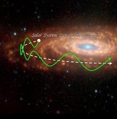 But maybe our own location isn’t always so habitable, either. It’s been observed that if you plot the number of extant species as a function of time on Earth (a biodiversity curve), there is a certain cyclicity to the peaks and troughs. Fourier analysis identifies frequencies that have a strong correlation with the signal. It was previously thought that there was a 26-27 Myr periodicity, but this is now viewed as an artifact of the sampling rate (through time) of the curve. After the recent revision of the geological time scale, a stronger signal is found with a period of 62 Myr. So, what might be happening to cause biodiversity to peak and fall every 62 Myr? There are a lot of ideas, including the Nemesis theory of a companion star repeatedly passing through and disrupting the solar system, a sharp increase in the number of mantle plumes in the Earth, solar nuclear oscillations, and, intriguingly, oscillations in the position of the solar system with respect to the galactic plane. We seem to rise up (“north”) of the galactic plane and dip down (“south”) with a period of about 64 Myr, which could be a potential match. When we head north, we move in “front” of the galaxy as it travels through the intergalactic medium, exposing us to more of the incoming cosmic rays, which are known to have negative effects on life. Three of the five known mass extinctions in history coincide with a peak of this vertical oscillation (one is already quite firmly believed to have been caused by a meteor impact and therefore need not fit with the cosmic ray periodicity). A less exotic explanation for the cyclicity is that sea level changes have affected how well fossils are preserved, therefore making it appear that there are fewer of them when preservation rates are low. In fact, strontium isotope ratios, which indicate the degree of rock weathering and erosion going on, seem to have a strong 59 My periodicity. I’d say that the jury’s still out on this one.
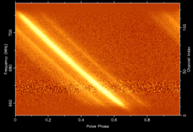 It turns out that pulsars, at least distant ones, do not manifest themselves as a blink of bright light (radiation). While presumably the signal starts out at a single frequency, over long distances it suffers dispersion that smears the pulse out over a range of frequencies. Even worse, the arrival time also gets smeared, so the higher frequencies arrive first and then “slide” down towards the lower ones (see example at right, taken from this handy explanation of pulsar dispersion). This means that if you aren’t sweeping frequencies at just the right time, you might totally miss a pulsar signal. The SKA will be hunting for these. Astronomers are particularly eager to find pulsars close to black holes, because pulsars are extremely reliable clocks and you should be able to test some interesting relativity hypotheses with a pulsar that’s within the black hole’s distortion field. (Related: see this ultra-cool animation of a recently discovered pulsar pair.)